A friend left this behind when they moved countries (knowing that I liked maths). This was my second attempt at reading it.
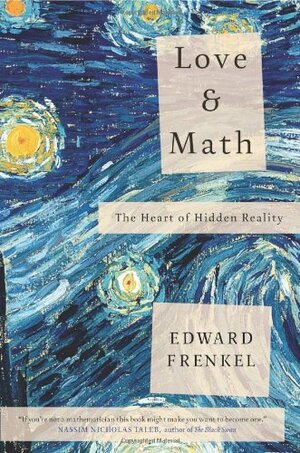
Here’s the blurb …
What if you had to take an art class in which you were only taught how to paint a fence? What if you were never shown the paintings of van Gogh and Picasso, weren’t even told they existed? Alas, this is how math is taught, and so for most of us it becomes the intellectual equivalent of watching paint dry.
In Love and Math , renowned mathematician Edward Frenkel reveals a side of math we’ve never seen, suffused with all the beauty and elegance of a work of art. In this heartfelt and passionate book, Frenkel shows that mathematics, far from occupying a specialist niche, goes to the heart of all matter, uniting us across cultures, time, and space.
Love and Math tells two intertwined stories: of the wonders of mathematics and of one young man’s journey learning and living it. Having braved a discriminatory educational system to become one of the twenty-first century’s leading mathematicians, Frenkel now works on one of the biggest ideas to come out of math in the last 50 years: the Langlands Program. Considered by many to be a Grand Unified Theory of mathematics, the Langlands Program enables researchers to translate findings from one field to another so that they can solve problems, such as Fermat’s last theorem, that had seemed intractable before.
At its core, Love and Math is a story about accessing a new way of thinking, which can enrich our lives and empower us to better understand the world and our place in it. It is an invitation to discover the magic hidden universe of mathematics.
I believe the aim of this book was to show non-maths people the beauty and joy of mathematics. However, I think it would be hard going if you didn’t have a mathematics background. This is high level mathematics (at one stage he mentions that there are probably about 12 people in the world who understand what he is discussing). Having said that, I liked it. I particularly liked the personal aspects of the narrative – his life experiences, and the people he met and with whom he worked.
I usually choose to use synthetic division when factorising polynomials, but I know some teachers are unhappy when their students do this. So for completeness, here is my PDF for Polynomial Long Division.
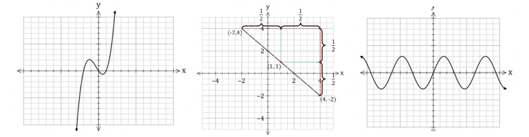
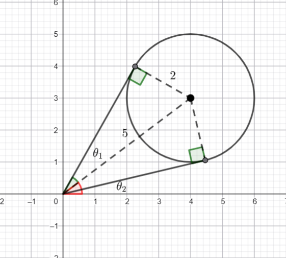
 is shown above, determine the maximum value of
  correct to two decimal places where
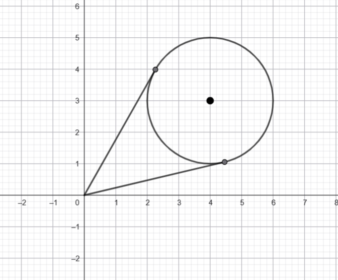
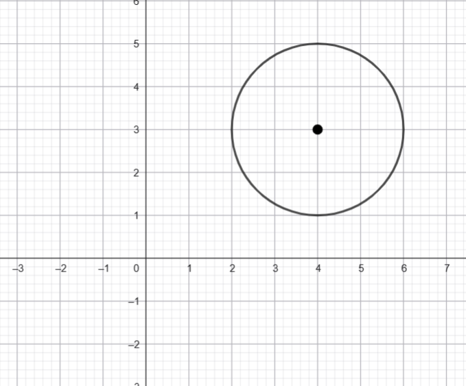
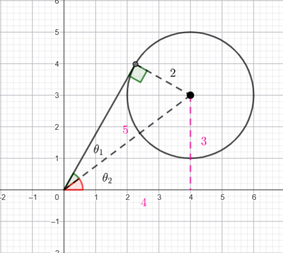
 and the centre is
  . Hence the distance from the origin to the centre is
  .
.


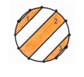
 and
and  have the same area.
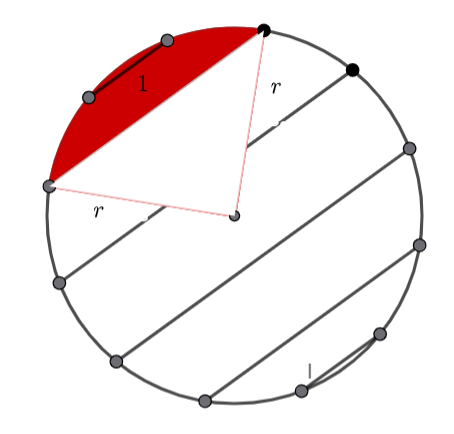

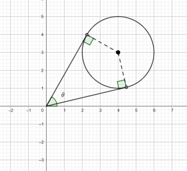
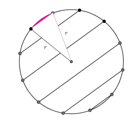
 where the angle measurement is in radians.


 equation


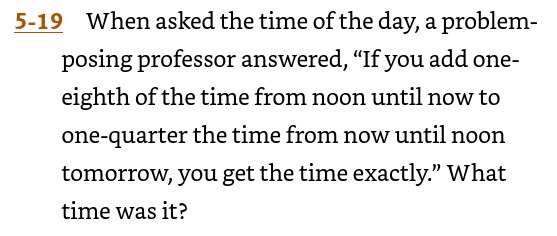
 be the number of hours from noon.
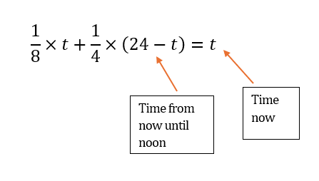


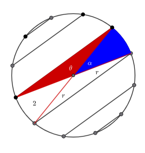
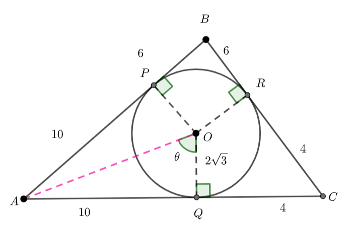
 and
and  subtract the sector
  .
.


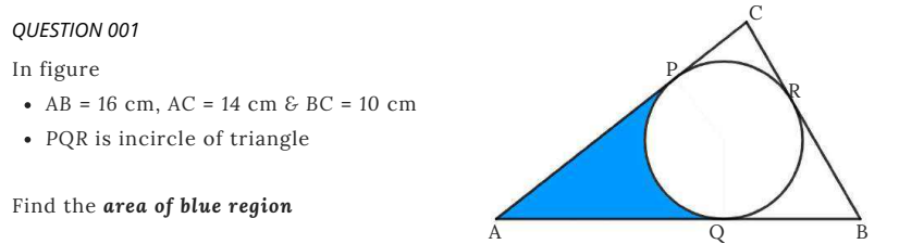
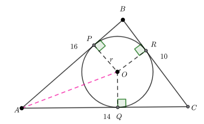
 where
where  is the radius of the inscribed circle.
 and
and 
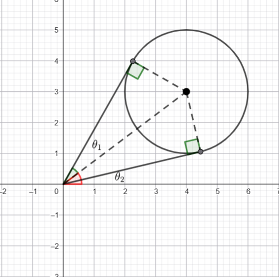
 , and
, and  – tangents to a circle are congruent.
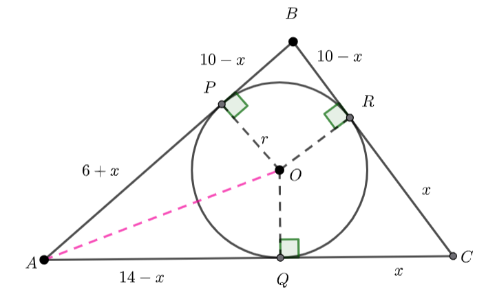


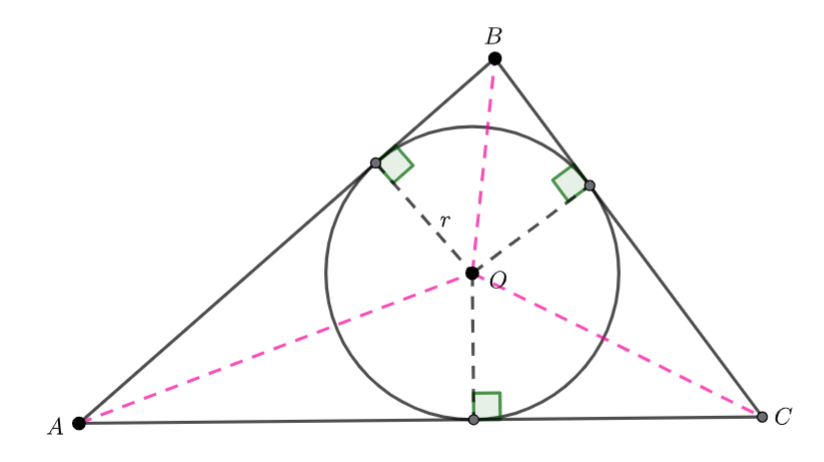
 Area
Area 


 is the semi-perimeter,
  and
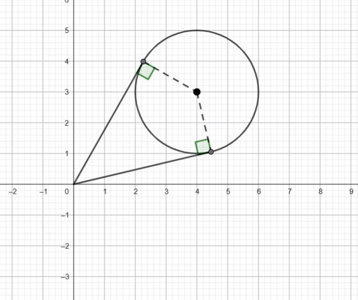
and  are tangents to the circle. And the radii are perpendicular to the tangents.
 and
and  .
.
 and
and  .
.


 for
for 


 or
or 

 for
for 


