Category Archives: Logistic Growth

March 26, 2025 · 12:23 pm

Logistic Growth Worked Example

A brumby is a free-roaming wild horse found in large number in parts of Australia. The culling of brumbies was banned in the year 2000. At this time the estimated population of brumbies in
Kosciuszko National Park was 1600. Scientists have modelled the population, P(t), of brumbies in
Kosciuszko National Park t years since the ban, by

$\begin{equation*}P(t)=\frac{18000}{10.25e^{0.15t}+1}\end{equation}$

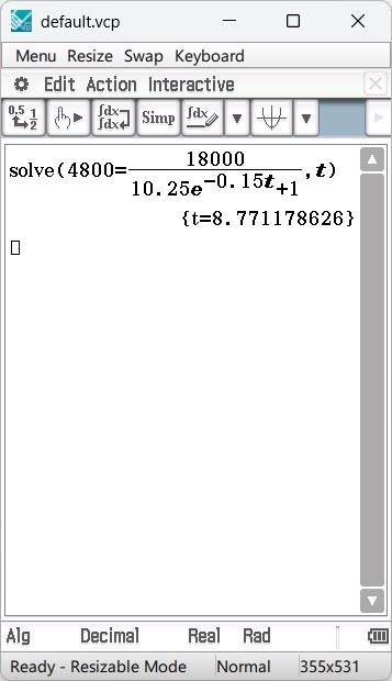
(a) Use the model to determine how long it will take the brumbies to increase to a number that is triple the number when the ban came into effect.

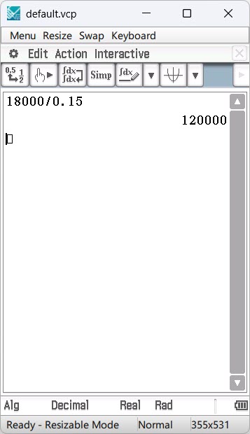
(b) From this model, determine the estimated long run number of brumbies in Kosciuszko National Park.

It can be shown that the growth rate of the population of brumbies can be expressed as

$\begin{equation*}\frac{dP}{dt}=\frac{1}{r}P(k-P)\end{equation}$

(d) Determine the greatest growth rate for the population of brumbies.

ATAR 2024 Specialist Mathematics Question 13

(a) $1600\times 3=4800$
$4800=\frac{18000}{10.25e^{0.15t}+1}$
$t=8.8$ years.

(b) $\lim_{\limits_{t \to \infty}\frac{18000}{10.25e^{0.15t}+1}=18000$

$\begin{equation*}\frac{dP}{dt}=rP(k-P)\Longleftrightarrow P=\frac{KP_0}{(k-P_0)e^{-rkt}+P_0}\end{equation}$

We have $\frac{1}{r}$ instead of $r$ .

Therefore,

$\begin{equation*}0.15=\frac{1}{r}\times 18000\end{equation}$

$r=120000$

(d) The greatest growth rate occurs when $P=\frac{k}{2}=9000$

$\begin{equation*}\frac{dP}{dt}=\frac{1}{r}P(k-P)\end{equation}$

$\begin{equation*}\frac{dP}{dt}=\frac{1}{120000}(9000)(9000)\end{equation}$

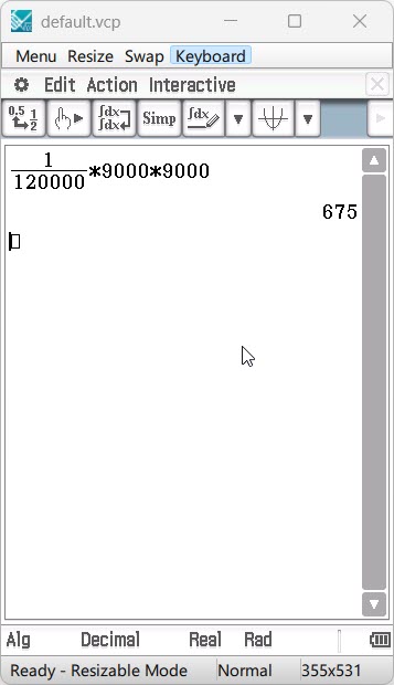
The greatest growth rate is 675 Brumbies per year.

1 Comment

Filed under Differential Equations, Logistic Growth, Year 12 Specialist Mathematics

Tagged as differential equations, logisitic growth, worked example, Year 12 Specialist Mathematics

March 25, 2025 · 7:32 am

Deriving the Logistic Growth Equation

The logistic differential equation

$\begin{equation*}\frac{dP}{dt}=rP(k-P)\end{equation}$

where $r$ is the growth parameter and $k$ is the carrying capacity.

And the maximum rate of increase happens when $P=\frac{k}{2}$

$\begin{equation*}\frac{dP}{dt}=rP(k-P)\end{equation}$

$\begin{equation*}\frac{dP}{P(k-P)}=r dt{\end{equation}$

$\begin{equation*}\int \frac{dP}{P(k-P)}=\int r dt{\end{equation}$

I am going to separate the denominator on the left hand side

\frac{1}{P(k-P)}=\frac{A}{P}+\frac{B}{k-P}

\frac{1}{P(k-P)}=\frac{A(k-P)+BP}{P(k-P)}

So our equation is,

$\begin{equation*}\int \frac{\frac{1}{k}}{P}+\frac{\frac{1}{k}}{k-P} dP=\int r dt\end{equation}$

$\begin{equation*}\frac{1}{k}\int \frac{1}{P}+\frac{1}{k-P} dP=\int r dt\end{equation}$

$\begin{equation*}\int \frac{1}{P}+\frac{1}{k-P} dP=\int kr dt\end{equation}$

$\begin{equation*}ln\lvert{P}\rvert-ln\lvert{k-P}\rvert=krt+c\end{equation}$

$\begin{equation*}ln\lvert{\frac{P}{k-P}\rvert=krt+c\end{equation}$

$\begin{equation*}\frac{P}{k-P}=e^{krt+c}\end{equation}$

$\begin{equation*}\frac{P}{k-P}=e^{krt}e^{c} \end{equation}$

When $t=0, P=P_0$ ,

$\begin{equation*}\frac{P_0}{k-P_0}=e^{c} \end{equation}$

The equation is now

$\begin{equation*}\frac{P}{k-P}=\frac{P_0}{k-P_0}e^{krt}\end{equation}$

$\begin{equation*}P=\frac{P_0}{k-P_0}e^{krt}(k-P)\end{equation}$

$\begin{equation*}P=k\frac{P_0}{k-P_0}e^{krt}-P\frac{P_0}{k-P_0}e^{krt}\end{equation}$

$\begin{equation*}P+P\frac{P_0}{k-P_0}e^{krt}=k\frac{P_0}{k-P_0}e^{krt}\end{equation}$

$\begin{equation*}P(1+\frac{P_0}{k-P_0}e^{krt})=k\frac{P_0}{k-P_0}e^{krt}\end{equation}$

$\begin{equation*}P=\frac{k\frac{P_0}{k-P_0}e^{krt}}{1+\frac{P_0}{k-P_0}e^{krt}}\end{equation}$

$\begin{equation*}P=\frac{k\frac{P_0}{k-P_0}e^{krt}}{\frac{k-P_0+P_0e^{krt}}{k-P_0}}\end{equation}$

$\begin{equation*}P=\frac{kP_0e^{rkt}}{k-P_0+P_0e^{rkt}}\end{equation}$

Divide by $e^{rkt}$

$\begin{equation*}P=\frac{kP_0}{(k-P_0)e^{-rkt}+P_0}\end{equation}$

$\begin{equation*}}\frac{dP}{dt}=rP(k-P)\Longleftrightarrow P=\frac{kP_0}{(k-P_0)e^{-rkt}+P_0}\end{equation}$

Proving the Maximum Rate of Increase Happens When $P=\frac{k}{2}$

$\begin{equation*}\frac{dP}{dt}=rP(k-P)\end{equation}$

$\begin{equation*}\frac{d^2P}{dt^2}=r\frac{dP}{dt}(k-P)+rP(-\frac{dP}{dt})\end{equation}$

$\begin{equation*}\frac{d^2P}{dt^2}=\frac{dP}{dt}(rk-rP-rP)\end{equation}$

$\begin{equation*}\frac{d^2P}{dt^2}=0\end{equation}$

$\begin{equation*}\frac{dP}{dt}(rk-rP-rP)=0\end{equation}$

$\begin{equation*}r\frac{dP}{dt}(k-2P)=0\end{equation}$

$\begin{equation*}\frac{dP}{dt}(k-2P)=0\end{equation}$

$\begin{equation*}rP(k-P)(k-2P)=0\end{equation}$

Hence $P=k$ or $P=\frac{k}{2}$

(1) $\begin{equation*}\frac{d^3P}{dt^3}=\frac{dP^2}{dt^2}(rk-2rP)+\frac{dP}{dt}(-2\frac{dP}{dt})\end{equation*}$

Substitute $P=k$ into equation $1$

$\begin{equation*}\frac{d^3P}{dt^3}=rk(k-k)(rk-2rk)(rk-2rk)-2(rk(k-k))^2=0\end{equation}$

Hence, not a maximum.

Substitute $P=\frac{k}{2}$ into equation $1$

$\begin{equation*}\frac{d^3P}{dt^3}=rk(k-\frac{k}{2})(rk-2r\frac{k}{2})(rk-2r\frac{k}{2})-2(rk(k-\frac{k}{2}))^2=0\end{equation}$

$\begin{equation*}\frac{d^3P}{dt^3}=-2(rk^2-\frac{rk^2}{2})^2\end{equation}$

$\begin{equation*}\frac{d^3P}{dt^3}=-2\frac{r^2k^4}{4}\end{equation}$

$-2\frac{r^2k^4}{4}\le 0$ For all values of $P, r$ and $k$ .

Hence maximum when $P=\frac{k}{2}$

We will look at a worked example in the next post.

The Logistic Equation

My year 12 Specialist students are working on logistic growth at the moment. An example might be helpful.

A new viral disease was found to spread according to the equation $\frac{dN}{dt}=kn(M-N)$ , where $M$ is the susceptible population, $N$ is the number of people infected at time $t$ months and $k=1.5\times 10^{-9}$ . In March 2010, it was thought only 100 people out of a population of 18 million were infected. Use the logistic model to find the number infected in:

(a) March 2011

(b) June 2012

(c) January 2017
Specialist 12 – Nelson Senior Maths